Visualisations make a Power BI report look great. Although they play a significant role in creating the first impression, businesses are always keen on the numbers or KPIs they convey. We build these numbers using a query language called DAX. In this blog, we will try to understand how table variables are correlated to the piping functions in R and Python.

Thank you for taking the time to read this blog. Let us dive right in.   

Problem Statement

The customer is interested in visualising a pie chart that displays the number of salespersons who contributed to the top 20%, middle 60%, and bottom 20% of the total Sales Amount for the chosen month and time period (MTD, YTD, etc.).  

To make it more transparent, let us take an example. Consider ten salespersons with ID 1 to 10, ID 1 having the highest sales, and 10 having the lowest deals. Let’s assume the total sale amount to be $100.   

If the sales amount of ID 1 is $20, then the number of salespersons contributed for the top 20% of the total sale amount is 1. If ID 1 and 2 together made a sale amount of $20 or greater than $20, then the number of salespersons contributed for the top 20% of the total sales amount is 2.   

To make it easy to understand the requirement, I mentioned that salespersons are in the order of the amount they sold; in the original data, this is not the case. We must sort the salespersons based on their sales amount before we compare the totals. The measure’s output will be the number of salespersons who contributed to the top 20% of the total sales amount.  Similarly, the last line of code is changed to obtain the middle 60% and the bottom 20%.  

In the following steps, we try to understand the above DAX code in multiple phases. 

Algorithm:  

Step 1 

Slicing the table based on the date and period selected (MTD, YTD, etc.) and adding the sales amount grouped by Salesperson and product division.  

Step 2 

Adding a column to the sliced table, which has rank values based on the Sum Amount  

Step 3 

The cumulative sum of the sales amount values is based on rank.  

Step 4 

In this step, we add a new column, Total_Sum, which is cum of all the values in the SUM_AMT column. 

Step 5

Number of salespersons contributing to the top 20% of the sales 

Detailed Explanation

Step 1 

Slicing the table based on the date and period selected and adding the sales amount grouped by Salesperson and product division.  

• The yellow part defines slicing the table based on the date; the green part defines the columns of the summarized table.  
•  The sum of the sales amount grouped by salesperson and category is aggregated in a new column, “SUM_AMT.” 

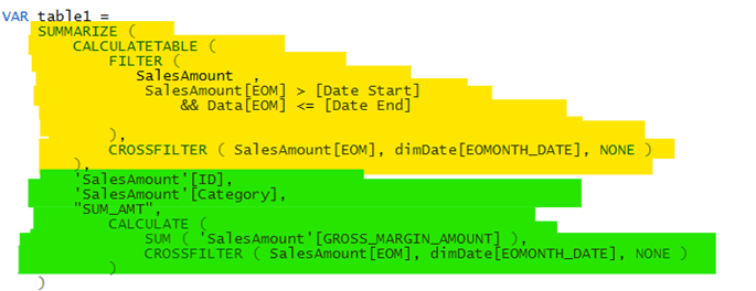
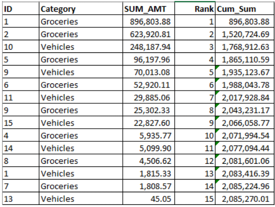
Below table is the output of the DAX in step 1. 

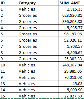
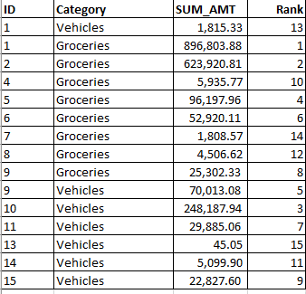
Step 2

Adding a column, “Rank,” to the table in step 1, each salesperson and category combination is ranked by “SUM_AMT.” 

• I added a new column to the table created in the previous step, which ranks the salesperson based on the SUM_AMT variable.  
• Skip is essential here because we use “Rank” in the next step to do a cumulative sum. When 5 values are tied with the same rank at 10, then the 6^th value will have a rank of 15 (10+5). 

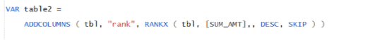
Step 3 

The cumulative sum of the SUM_AMT values based on rank  

• I added a new column, “CUM_SUM,” to the table created in the previous step.  

• We should note that DAX can only access table variables via iterative functions such as SUMX, RANKX, MAXX, etc. But not SUM or RANK-like functions which are not iterative. 
• The code below adds a column CUM_SUM whose values are the sum of topN rows of SUM_AMT; for the first row, it is equal to Max (SUM_AMT), for the second row, it is equal to the sum of the first two values of SUM_AMT. 

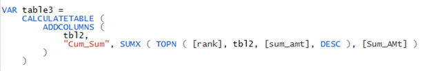
Step 4

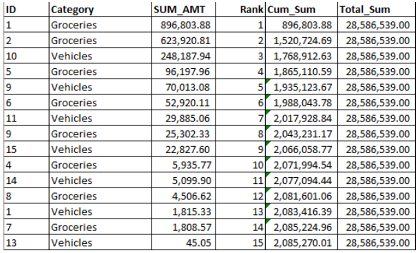
Add a new column, Total_Sum which is cum of all the values in the SUM_AMT column. 

Step 5  

Number of the salesperson contributing to the top 20% of the sales  

• Tbl4 in the code left adds column Total_Sum, which is the total Sum of Sum_Amt for all the salespersons.  
• We use this value to filter the table and count rows whose cumulative sum is less than or equal to 20% of the total sum (+-1 tolerance).  

• The same measure is repeated for multiple percentage values and used as values of the Pie Chart.  

The answer will be four, as the sum of the first four rows (rank 1 to 4) is greater than 20% of the total sum.  

Well, that is all of it. The same is repeated to obtain the middle 60% and bottom 20% count. A pie chart visual is added to the report, with all three measures which result in the picture below.   

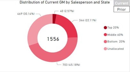
P.S. Unallocated is a different category apart from the three percentages. 

I have included the entire code below so that you can practice or use it.

Raghu Gorla

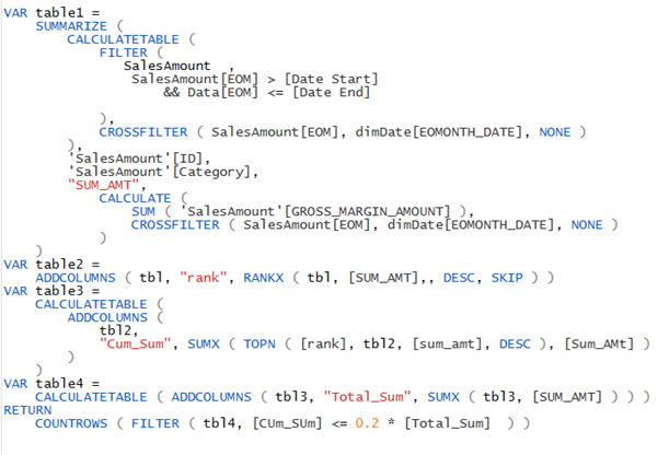
—- Code —-

Dax Measure for the top 20% is as below.

Evaluate

VAR table1 =

     SUMMARIZE (

         CALCULATETABLE (

             FILTER (

                SalesAmount  ,

                 SalesAmount[EOM] > [Date Start]

                     && Data[EOM] <= [Date End]

             ),

             CROSSFILTER ( SalesAmount[EOM], dimDate[EOMONTH_DATE], NONE )

         ),

         ‘SalesAmount'[ID],

         ‘SalesAmount'[Category],

         “SUM_AMT”,

             CALCULATE (

                 SUM ( ‘SalesAmount'[GROSS_MARGIN_AMOUNT] ),

                 CROSSFILTER ( SalesAmount[EOM], dimDate[EOMONTH_DATE], NONE )

             )

     )

 VAR table2 =

    ADDCOLUMNS ( tbl, “rank”, RANKX ( tbl, [SUM_AMT],, DESC, SKIP ) )

 VAR table3 =

     CALCULATETABLE (

         ADDCOLUMNS (

             tbl2,

             “Cum_Sum”, SUMX ( TOPN ( [rank], tbl2, [sum_amt], DESC ), [SUM_AMT] )

         )

     )

 VAR table4 =

    CALCULATETABLE ( ADDCOLUMNS ( tbl3, “Total_Sum”, SUMX ( tbl3, [SUM_AMT] ) ) )

RETURN

     COUNTROWS ( FILTER ( tbl4, [Cum_Sum] <= 0.2 * [Total_Sum]  ) )